Can MapReduce solve planning problems?
To solve a planning or optimization problem, some solvers tend to scale out poorly: As the problem has more variables and more constraints, they use a lot more RAM memory and CPU power. They can hit hardware memory limits at a few thousand variables and few million constraint matches. One way their users typically work around such hardware limits, is to use MapReduce. Let’s see what happens if we MapReduce a planning problem, such as the Traveling Salesman Problem.
About MapReduce
MapReduce is programming model which has proven to be very effective to run a query on big data. Generally speaking, it works like this:
- The data is partitioned across multiple computer nodes.
- A map function runs on every partition and returns a result.
- A reduce function reduces 2 results into one result. Its continuously run until only a single result remains.
For example, suppose we need to find the most expensive invoice record in a data cluster:
- The invoice records are partitioned across multiple computer nodes.
- For each node, the map function extracts the most expensive invoice for that node.
- The reduce function takes 2 invoices and returns the most expensive.
About the Traveling Salesman Problem
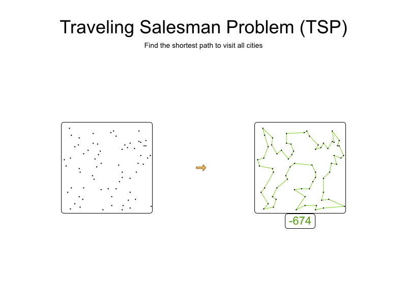
The Traveling Salesman Problem (TSP) is a very basic planning problem. Given a list of cities, find the shortest path to visit all cities.
For example, here’s a dataset with 68 cities and its optimal tour with a distance of 674:
The search space of this small dataset has 68 (= 1096) combinations. That’s a lot.
A more realistic planning problem, such vehicle routing, has more constraints (both in number as in complexity), such as: vehicle capacity, vehicle type limitations, time windows, driver limits, etc.
MapReduce on TSP
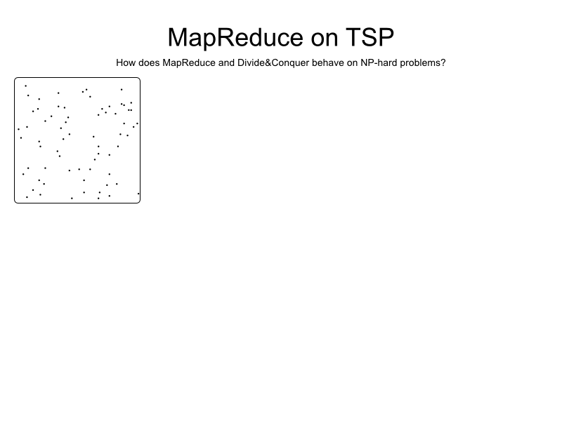
Even though most solvers probably won’t go out of memory on only 68 variables, the small size of this problem allows us to visualize it clearly:
Let’s apply MapReduce on it:
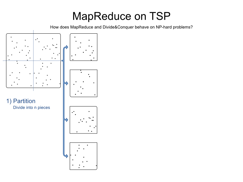
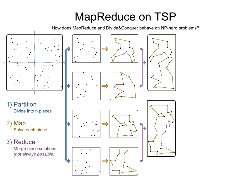
1) Partition: Divide the problem into n pieces
First, we take the problem and split it into n pieces. Usually, n is the number of computer nodes in our system. For visual reasons, we divide it into only 4 pieces:
TSP is easily partitioned because of it only has 1 relevant constraint: find the shortest path.
In a more realistic planning problem, sane partitioning can be hard or even impossible. For example:
- In capacitated vehicle routing, no 2 partitions should share the same vehicle. What if we have more partitions than vehicles?
- In vehicle routing with time windows, each partition should have enough vehicle time to service each customer and drive to each location. Catch 22: How do we determine the drive time if we don’t know the vehicle routes yet?
It’s tempting to make false assumptions.
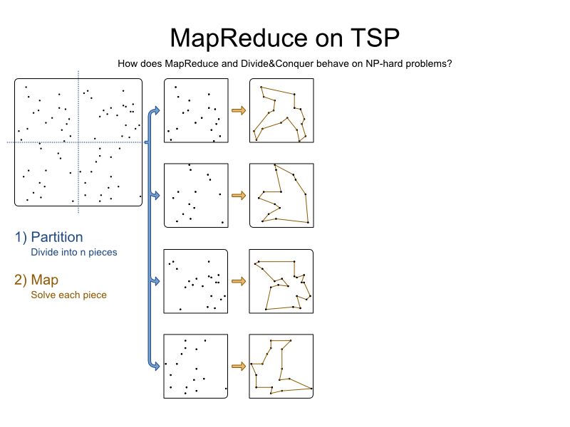
2) Map: Solve each piece separately
Solve each partition using a Solver:
We get 4 pieces, each with a partial solution.
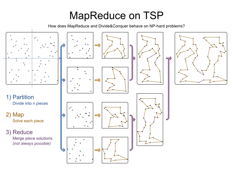
3) Reduce: Merge solution pieces
Merge the pieces together. To merge 2 pieces together, we remove an arc from each piece and add 2 arcs to connect cities of different pieces:
We do merge several times until all pieces are merged:
There are several ways to merge 2 pieces together. Here we try every combination and take the optimal one. For performance reasons, we might instead connect the 2 closest cities of different pieces with an arc, and then add a correcting arc on the other side (however long that may be).
In a more realistic planning problem, with more complex constraints, merging feasible partial solutions often results into an infeasible solution (with broken hard constraints). Smarter partitioning, which takes all the hard constraints into account, can sometimes solve this… at the expense of more broken soft constraints and a higher maintenance cost.
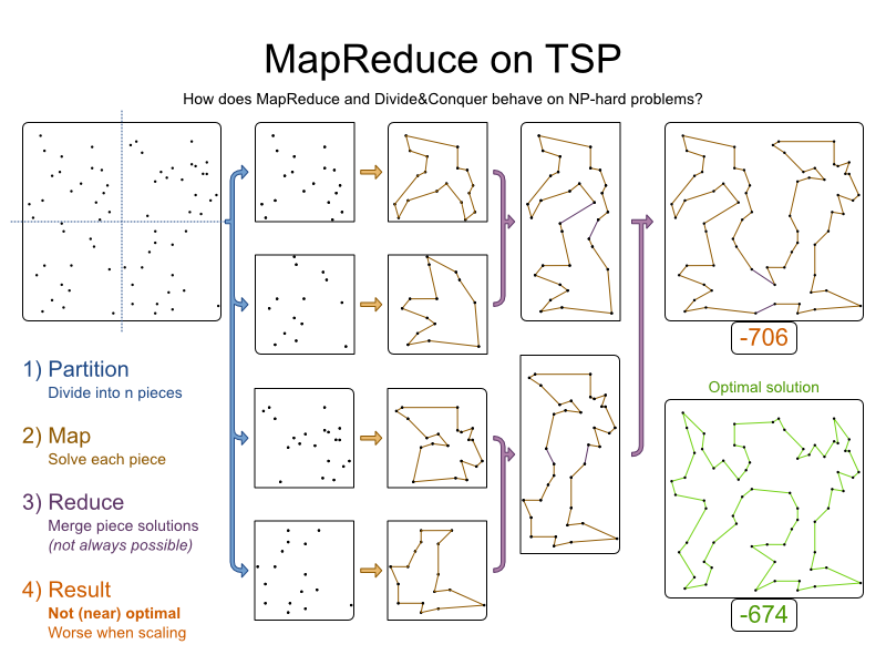
4) Result: What is the quality of the result?
Each piece was solved optimally. Pieces were merged optimally. But the result is not optimal:
In fact, the results aren’t even near optimal, especially as we scale out with a MapReduce approach:
- More variables result in a lower result quality.
- More constraints result in a lower result quality, presuming it’s even possible to partition and reduce sanely.
- More partitions, result in a lower result quality.
Conclusion
MapReduce is great approach to handle a query problem (and presumably many other problems). But MapReduce is a terrible approach on a planning or optimization problem. Use the right tool for the job.
Note: We applied MapReduce on the planning problem, not on the optimization algorithm implementation in a Solver, for which it can make sense. For example, in a depth-first search algorithm, MapReduce can make sense to explore the search tree (although the search tree scales exponentially bad which dwarfs any gain of MapReduce).
To solve a big planning problem, use a Solver (such as OptaPlanner) that scales well in memory, so you don’t to resort to partitioning at the expense of solution quality.

