R: Snakes and ladders markov chain
A few days ago I read a really cool blog post explaining how Markov chains can be used to model the possible state transitions in a game of snakes and ladders, a use of Markov chains I hadn’t even thought of!
While the example is very helpful for understanding the concept, my understanding of the code is that it works off the assumption that any roll of the dice that puts you on a score > 100 is a winning roll.
In the version of the game that I know you have to land exactly on 100 to win. e.g if you’re on square 98 and roll a 6 you would go forward 2 spaces to 100 and then bounce back 4 spaces to 96.
I thought it’d be a good exercise to tweak the code to cater for this:
n=100

# We have 6 extra columns because we want to represent throwing of the dice which results in a final square > 100
M=matrix(0,n+1,n+1+6)
rownames(M)=0:n
colnames(M)=0:(n+6)

# set probabilities of landing on each square assuming that there aren't any snakes or ladders
for(i in 1:6){
  diag(M[,(i+1):(i+1+n)])=1/6
}

# account for 'bounce back' if a dice roll leads to a final score > 100
for(i in 96:100) {
  for(c in 102:107) {
    idx = 101 - (c - 101)
    M[i, idx] = M[i, idx] + M[i, c]
  }
}
We can inspect the last few rows to check that if the transition matrix is accurate:
> M[95:100,95:101]

   94        95        96        97        98        99       100
94  0 0.1666667 0.1666667 0.1666667 0.1666667 0.1666667 0.1666667
95  0 0.0000000 0.1666667 0.1666667 0.1666667 0.3333333 0.1666667
96  0 0.0000000 0.0000000 0.1666667 0.3333333 0.3333333 0.1666667
97  0 0.0000000 0.0000000 0.1666667 0.3333333 0.3333333 0.1666667
98  0 0.0000000 0.1666667 0.1666667 0.1666667 0.3333333 0.1666667
99  0 0.1666667 0.1666667 0.1666667 0.1666667 0.1666667 0.1666667
If we’re on the 99th square (the last row) we could roll a 1 and end up on 100, a 2 and end up on 99 (1 forward, 1 back), a 3 and end up on 98 (1 forward, 2 back), a 4 and end up on 97 (1 forward, 3 back), a 5 and end up on 96 (1 forward, 4 back) or a 6 and end up on 95 (1 forward, 5 back). i.e. we can land on 95, 96, 97, 98, 99 or 100 with 1/6 probability.
If we’re on the 96th square (the 3rd row) we could roll a 1 and end up on 97, a 2 and end up on 98, a 3 and end up on 99, a 4 and end up on 100, a 5 and end up on 99 (4 forward, 1 back) or a 6 and end up on 98 (4 forward, 2 back). i.e. we can land on 97 with 1/6 probability, 98 with 2/6 probability, 99 with 2/6 probability or 100 with 1/6 probability.
We could do a similar analysis for the other squares but it seems like the probabilities are being calculated correctly.
Next we can update the matrix with the snakes and ladders. That code stays the same:
# get rid of the extra columns, we don't need them anymore
M=M[,1:(n+1)]

# add in the snakes and ladders
starting = c(4,9,17,20,28,40,51,54,62,64,63,71,93,95,92)
ending   = c(14,31,7,38,84,59,67,34,19,60,81,91,73,75,78)

for(i in 1:length(starting)) {
  # Retrieve current probabilities of landing on the starting square
  v=M[,starting[i]+1]
  ind=which(v>0)

  # Set no probability of falling on the starting squares
  M[ind,starting[i]+1]=0

  # Move all existing probabilities to the ending squares
  M[ind,ending[i]+1]=M[ind,ending[i]+1]+v[ind]
}
We can also simplify the powermat function which is used to simulate what the board would look like after a certain number of dice rolls:
# original
powermat=function(P,h){
  Ph=P
  if(h>1) {
    for(k in 2:h) {
      Ph=Ph%*%P
    }
  }
  return(Ph)
}

#new
library(expm)
powermat = function(P,h) {
  return (P %^% h)
}
initial=c(1,rep(0,n))
h = 1
> (initial%*%powermat(M,h))[1:15]
0 1 2 3 4 5 6 7 8 9 10 11 12 13 14 15 16 17 18 19 20 21 22 23 24 25 26 27 28 29 30 31 32 33 34 35 36 37 38 39 40 41 42 43 44 45
[1,] 0 0.1666667 0.1666667 0.1666667 0 0.1666667 0.1666667 0 0 0 0 0 0 0 0.1666667 0 0 0 0 0 0 0 0 0 0 0 0 0 0 0 0 0 0 0 0 0 0 0 0 0 0 0 0 0 0 0
46 47 48 49 50 51 52 53 54 55 56 57 58 59 60 61 62 63 64 65 66 67 68 69 70 71 72 73 74 75 76 77 78 79 80 81 82 83 84 85 86 87 88 89 90 91 92 93 94 95 96 97 98 99 100
[1,] 0 0 0 0 0 0 0 0 0 0 0 0 0 0 0 0 0 0 0 0 0 0 0 0 0 0 0 0 0 0 0 0 0 0 0 0 0 0 0 0 0 0 0 0 0 0 0 0 0 0 0 0 0 0 0One interesting thing I noticed is that it now seems to take way more turns on average to finish the game than when you didn’t need to score exactly 100 to win:
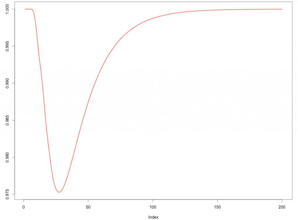
> sum(1 - game)
[1] 999
distrib=initial%*%M
game=rep(NA,1000)
for(h in 1:length(game)){
game[h]=distrib[n+1]
distrib=distrib%*%M}
plot(1-game[1:200],type="l",lwd=2,col="red",
ylab="Probability to be still playing")
I expected it to take longer to finish the game but not this long! I think I’ve probably made a mistake but I’m not sure where…
Update
Antonios found the mistake I’d made – when on the 100th square we should have a 1 as the probability of getting to the 100th square. i.e. we need to update M like so:
M[101,101] = 1
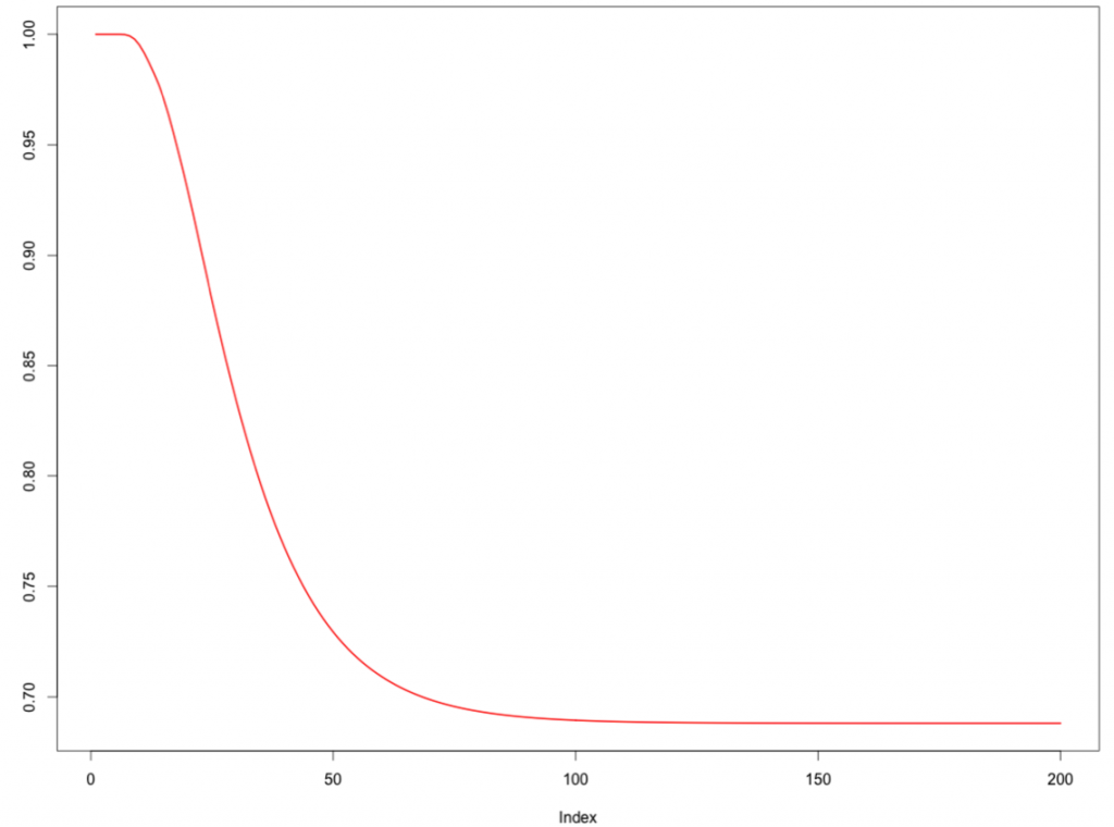
Now if we visualise he probability that we’re still playing we get a more accurate curve:
distrib=initial%*%M
game=rep(NA,1000)
for(h in 1:length(game)){
game[h]=distrib[n+1]
distrib=distrib%*%M}
plot(1-game[1:200],type="l",lwd=2,col="red",
ylab="Probability to be still playing")| Reference: | R: Snakes and ladders markov chain from our JCG partner Mark Needham at the Mark Needham Blog blog. |


