A Brief Overview of Performance Enhancements in Apache Drill 1.4

Neeraja RentachintalaJanuary 18th, 2016Last Updated: January 17th, 2016

0 33 10 minutes read

Today we are excited to announce that Apache Drill 1.4 is now available on the MapR Distribution. Drill 1.4 is a production-ready and supported version on MapR and can be downloaded from here and find the 1.4 release notes here.

Building on the foundation of its highly flexible and scale-out architecture, Drill 1.4 brings a variety of new features as well as enhancements to the query performance, making it a very important milestone for the Drill community.

Here is a list of key features/enhancements available in Drill 1.4.

Improved Tableau experience with faster Limit 0 queries
Metadata (INFORMATION_SCHEMA) query speed-ups on Hive schemas/tables
Optimized query planning and execution through enhanced partition pruning
Efficient caching of Parquet metadata, speeding up queries on large numbers of files
Improved window functions, resource usage, and performance
Table functions
Improved CSV header parsing
New and improved MapR Drill JDBC driver

In this blog post, I want to specifically provide a quick overview of a couple of recent performance enhancements, namely partition pruning and Parquet metadata caching, that will enable you to achieve low latency response times in your Drill deployments. Metadata caching is a new feature added in Drill 1.2 and partition pruning existed since Drill 1.0, but with 1.4, both of these features are much more efficient and cover a broad spectrum of use cases.

Let me start with some background. Drill is designed to achieve interactive performance on large-scale datasets containing a wide variety of data types and data sources. Performance in any query engine is comprised of two parts:

The time spent in parsing the query and creating the most optimal query plan (a.k.a. query planning time).
The time spent in executing the generated query plan across various nodes in the cluster by retrieving and processing the data from the underlying storage system (a.k.a query execution time).

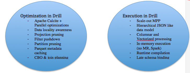
Below is a list of some of the core Drill architecture elements and techniques at each of these phases that enable Drill to achieve the interactive performance. As you can see, both partition pruning and metadata caching are examples of optimization techniques that are applied as part of query planning.

Partition pruning

Dataset sizes in big data systems such as Hadoop can be monumental, ranging from terabytes to petabytes. In some cases, the datasets might start small, but customers choose Hadoop because they expect data volume to grow significantly and pretty rapidly. Partition pruning allows a query engine to be able to determine and retrieve the smallest needed dataset to answer a given query. Reading small data means fewer cycles on the IO and fewer cycles on the CPU to actually process data. This is a standard technique applied in traditional DBMS/MPP systems to achieve performance, but becomes much more critical in the context of big data due to the large volumes of data. In order to leverage partition pruning as part of queries, the data needs to be organized and partitioned appropriately based on the patterns of queries you expect to get from the users.

Organizing data can be done at ingestion time or done subsequently as a processing step by using a variety of Hadoop ecosystem tools such as Flume, Hive, Pig, or through direct ingestion via NFS, in the case of MapR. Drill supports partition pruning with various types of storage plugins. Partition pruning is applied when querying file systems based on the directory structure of files and using Hive metastore table partition information when querying Hive tables. Drill itself provides the ability to create partitioned data as part of the CREATE TABLE AS syntax.

Here is an example of partitioning data using Drill SQL syntax. This statement converts a sample Yelp business JSON dataset (which can be downloaded from Yelp) to the Parquet format. As part of the conversion, data is also partitioned based on three columns, namely state, city, and stars.

0: jdbc:drill:zk=local> create table dfs.tmp.businessparquet partition by (state,city,stars) as select state, city, stars, business_id, full_address, hours,name, review_count from `business.json`;

The output of the above statement is Parquet data that was generated in a directory corresponding to a specified workspace. In this case, dfs.tmp workspace points to /tmp location on the file system and the generated directory is /tmp/businessparquet, which is the table name specified in the SQL clause.

Let’s get the number of files generated by CTAS command.

NRentachintala-MAC:businessparquet nrentachintala$ cd /tmp/businessparquet/ 

NRentachintala-MAC:businessparquet nrentachintala$ ls -l |wc -l
     652

Note the number of files generated by the Drill CTAS command can be tuned with a variety of parameters in Drill; however, the default matches the number of distinct combinations the partition key columns specified in CTAS will have. For example, the following SQL statement gives you the number of distinct combinations of partition key columns.

0: jdbc:drill:zk=local> select count(*) from (select distinct state, city, stars from dfs.yelp.`business.json`) ;
+---------+
| EXPR$0  |
+---------+
| 652     |
+---------+

Now that the Parquet data is partitioned, queries coming in with filters on partition columns (state, city, stars) can leverage the partition pruning optimization; only the relevant data is read from the disk and the remaining partitions are pruned out at planning time.

You can easily check whether partition pruning is applied or not for a given query by running the EXPLAIN PLAN command on the query, or viewing the profiles from the Drill web UI (which can be launched from 8047 port from the Drillbit node).

Let’s take a couple of sample queries and see whether partition pruning is applied using the web UI.

Here is one query with filters on two of the partition columns—state and city.

0: jdbc:drill:zk=local> select name, city, stars from dfs.tmp.businessparquet where state='AZ' and city = 'Fountain Hills' limit 5;

+-----------------------------------------------+-----------------+--------+
|                     name                      |      city       | stars  |
+-----------------------------------------------+-----------------+--------+
| Fry's Food & Drug Stores                      | Fountain Hills  | 2.0    |
| Burger King                                   | Fountain Hills  | 2.0    |
| Francis & Sons Car Wash                       | Fountain Hills  | 2.0    |
| Kimmies                                       | Fountain Hills  | 2.0    |
| Le Baron Cleaners At Basha's Shopping Center  | Fountain Hills  | 3.5    |
+-----------------------------------------------+-----------------+--------+
5 rows selected (0.308 seconds)

The physical query plan looks like the following in the web UI for this query. Note the highlighted ‘numFiles’ value in the profile. This represents how many files are read off of disk to serve the query. In this case, 9 files out of 652 are read because the query applies filters on both state and city columns that are partition keys, and prunes out the remaining partitions of data. Checking # of files read is a simple way to ensure whether partition is applied.

00-00    Screen : rowType = RecordType(ANY name, ANY city, ANY stars): rowcount = 5.0, cumulative cost = {129.5 rows, 501.5 cpu, 0.0 io, 0.0 network, 0.0 memory}, id = 731
00-01      Project(name=[$0], city=[$1], stars=[$2]) : rowType = RecordType(ANY name, ANY city, ANY stars): rowcount = 5.0, cumulative cost = {129.0 rows, 501.0 cpu, 0.0 io, 0.0 network, 0.0 memory}, id = 730
00-02        SelectionVectorRemover : rowType = RecordType(ANY name, ANY city, ANY stars): rowcount = 5.0, cumulative cost = {129.0 rows, 501.0 cpu, 0.0 io, 0.0 network, 0.0 memory}, id = 729
00-03          Limit(fetch=[5]) : rowType = RecordType(ANY name, ANY city, ANY stars): rowcount = 5.0, cumulative cost = {124.0 rows, 496.0 cpu, 0.0 io, 0.0 network, 0.0 memory}, id = 728
00-04            Limit(fetch=[5]) : rowType = RecordType(ANY name, ANY city, ANY stars): rowcount = 5.0, cumulative cost = {119.0 rows, 476.0 cpu, 0.0 io, 0.0 network, 0.0 memory}, id = 727
00-05              Project(name=[$2], city=[$1], stars=[$3]) : rowType = RecordType(ANY name, ANY city, ANY stars): rowcount = 114.0, cumulative cost = {114.0 rows, 456.0 cpu, 0.0 io, 0.0 network, 0.0 memory}, id = 726
00-06                Project(state=[$1], city=[$2], name=[$0], stars=[$3]) : rowType = RecordType(ANY state, ANY city, ANY name, ANY stars): rowcount = 114.0, cumulative cost = {114.0 rows, 456.0 cpu, 0.0 io, 0.0 network, 0.0 memory}, id = 725
00-07                  Scan(groupscan=[ParquetGroupScan [entries=[ReadEntryWithPath [path=/tmp/businessparquet/0_0_111.parquet], ReadEntryWithPath [path=/tmp/businessparquet/0_0_114.parquet], ReadEntryWithPath [path=/tmp/businessparquet/0_0_115.parquet], ReadEntryWithPath [path=/tmp/businessparquet/0_0_110.parquet], ReadEntryWithPath [path=/tmp/businessparquet/0_0_109.parquet], ReadEntryWithPath [path=/tmp/businessparquet/0_0_113.parquet], ReadEntryWithPath [path=/tmp/businessparquet/0_0_116.parquet], ReadEntryWithPath [path=/tmp/businessparquet/0_0_117.parquet], ReadEntryWithPath [path=/tmp/businessparquet/0_0_112.parquet]], selectionRoot=file:/tmp/businessparquet, numFiles=9, usedMetadataFile=false, columns=[`state`, `city`, `name`, `stars`]]]) : rowType = RecordType(ANY name, ANY state, ANY city, ANY stars): rowcount = 114.0, cumulative cost = {114.0 rows, 456.0 cpu, 0.0 io, 0.0 network, 0.0 memory}, id = 724

Now let’s extend the above query by adding another filter with the stars column, which is a partition key as well.

0: jdbc:drill:zk=local> select name, city, stars from dfs.tmp.businessparquet where state='AZ' and city = 'Fountain Hills' and stars= '3.5' limit 5;
+-----------------------------------------------+-----------------+--------+
|                     name                      |      city       | stars  |
+-----------------------------------------------+-----------------+--------+
| Le Baron Cleaners At Basha's Shopping Center  | Fountain Hills  | 3.5    |
| Euro Pizza Cafe                               | Fountain Hills  | 3.5    |
| Deluxe Nail & Spa                             | Fountain Hills  | 3.5    |
| Ha Ha China                                   | Fountain Hills  | 3.5    |
| Pony Express                                  | Fountain Hills  | 3.5    |
+-----------------------------------------------+-----------------+--------+
5 rows selected (0.342 seconds)

Notice the physical plan for this query as below shows ‘numFiles’ as just 1. So Drill had to read just 1 out of 652 files to answer the query. The more partition-based filters you have in the query, the more the query can be pointed towards the very specific subset of the data. This could lead to huge performance improvements. Note, however, that your query might be extremely complex, in which case the performance benefits obtained from partition pruning may not be comparable to the processing cost of the query. However, in most of the simple and medium queries, this will be a great help. Also, the most important aspect of leveraging partition pruning is figuring out the common query patterns and partitioning the data accordingly. Spend some time on this to tune your deployment.

00-00    Screen : rowType = RecordType(ANY name, ANY city, ANY stars): rowcount = 5.0, cumulative cost = {40.5 rows, 145.5 cpu, 0.0 io, 0.0 network, 0.0 memory}, id = 1005
00-01      Project(name=[$0], city=[$1], stars=[$2]) : rowType = RecordType(ANY name, ANY city, ANY stars): rowcount = 5.0, cumulative cost = {40.0 rows, 145.0 cpu, 0.0 io, 0.0 network, 0.0 memory}, id = 1004
00-02        SelectionVectorRemover : rowType = RecordType(ANY name, ANY city, ANY stars): rowcount = 5.0, cumulative cost = {40.0 rows, 145.0 cpu, 0.0 io, 0.0 network, 0.0 memory}, id = 1003
00-03          Limit(fetch=[5]) : rowType = RecordType(ANY name, ANY city, ANY stars): rowcount = 5.0, cumulative cost = {35.0 rows, 140.0 cpu, 0.0 io, 0.0 network, 0.0 memory}, id = 1002
00-04            Project(name=[$3], city=[$1], stars=[$2]) : rowType = RecordType(ANY name, ANY city, ANY stars): rowcount = 30.0, cumulative cost = {30.0 rows, 120.0 cpu, 0.0 io, 0.0 network, 0.0 memory}, id = 1001
00-05              Project(state=[$1], city=[$2], stars=[$3], name=[$0]) : rowType = RecordType(ANY state, ANY city, ANY stars, ANY name): rowcount = 30.0, cumulative cost = {30.0 rows, 120.0 cpu, 0.0 io, 0.0 network, 0.0 memory}, id = 1000
00-06                Scan(groupscan=[ParquetGroupScan [entries=[ReadEntryWithPath [path=/tmp/businessparquet/0_0_114.parquet]], selectionRoot=file:/tmp/businessparquet, numFiles=1, usedMetadataFile=false, columns=[`state`, `city`, `stars`, `name`]]]) : rowType = RecordType(ANY name, ANY state, ANY city, ANY stars): rowcount = 30.0, cumulative cost = {30.0 rows, 120.0 cpu, 0.0 io, 0.0 network, 0.0 memory}, id = 999

Parquet metadata caching

Another common characteristic of Hadoop deployments is the number of files on the file system. We have seen customers use Drill to query hundreds of thousands to millions of files, both for reporting and ETL use cases. One of the differentiating capabilities of Drill is its ability to work with self-describing data formats such as Parquet, and discovering the schema on-the-fly. Parquet stores the metadata about the data as part of file footers, and it includes information such as column names, data types, nullability, and other column characteristics as well as parameters around the layout of data such as row group size. This information is leveraged by Drill as part of the planning time. While Drill has ability to discovery this metadata at the query time, this could be an expensive operation for the use cases where there are many files. Starting from Drill 1.2, we introduced a capability to cache Parquet metadata in Drill. Once metadata is cached, it can be refreshed as needed, depending on how frequently the datasets change in the environment.

Below is the command to use cache metadata. The command can be used for a folder or a single file.

0: jdbc:drill:zk=local> REFRESH TABLE METADATA dfs.tmp.BusinessParquet;
+-------+-----------------------------------------------------------+
|  ok   |                          summary                          |
+-------+-----------------------------------------------------------+
| true  | Successfully updated metadata for table BusinessParquet.  |
+-------+-----------------------------------------------------------+
1 row selected (0.455 seconds)

The query profile in the web UI or the Explain Plan command showcases whether metadata cache is leveraged for a given query.

0: jdbc:drill:zk=local> select name, city, stars from dfs.tmp.businessparquet where state='AZ' and city = 'Fountain Hills' and stars= '3.5' limit 5;

Note that the highlighted ‘usedMetadataCacheFile=true’ in the following profile indicates that metadata caching is leveraged for this command.

00-00    Screen : rowType = RecordType(ANY name, ANY city, ANY stars): rowcount = 5.0, cumulative cost = {40.5 rows, 145.5 cpu, 0.0 io, 0.0 network, 0.0 memory}, id = 1279
00-01      Project(name=[$0], city=[$1], stars=[$2]) : rowType = RecordType(ANY name, ANY city, ANY stars): rowcount = 5.0, cumulative cost = {40.0 rows, 145.0 cpu, 0.0 io, 0.0 network, 0.0 memory}, id = 1278
00-02        SelectionVectorRemover : rowType = RecordType(ANY name, ANY city, ANY stars): rowcount = 5.0, cumulative cost = {40.0 rows, 145.0 cpu, 0.0 io, 0.0 network, 0.0 memory}, id = 1277
00-03          Limit(fetch=[5]) : rowType = RecordType(ANY name, ANY city, ANY stars): rowcount = 5.0, cumulative cost = {35.0 rows, 140.0 cpu, 0.0 io, 0.0 network, 0.0 memory}, id = 1276
00-04            Project(name=[$3], city=[$1], stars=[$2]) : rowType = RecordType(ANY name, ANY city, ANY stars): rowcount = 30.0, cumulative cost = {30.0 rows, 120.0 cpu, 0.0 io, 0.0 network, 0.0 memory}, id = 1275
00-05              Project(state=[$1], city=[$2], stars=[$3], name=[$0]) : rowType = RecordType(ANY state, ANY city, ANY stars, ANY name): rowcount = 30.0, cumulative cost = {30.0 rows, 120.0 cpu, 0.0 io, 0.0 network, 0.0 memory}, id = 1274
00-06                Scan(groupscan=[ParquetGroupScan [entries=[ReadEntryWithPath [path=/tmp/BusinessParquet/0_0_114.parquet]], selectionRoot=/tmp/BusinessParquet, numFiles=1, usedMetadataFile=true, columns=[`state`, `city`, `stars`, `name`]]]) : rowType = RecordType(ANY name, ANY state, ANY city, ANY stars): rowcount = 30.0, cumulative cost = {30.0 rows, 120.0 cpu, 0.0 io, 0.0 network, 0.0 memory}, id = 1273

The combination of partition pruning and metadata caching can result in huge performance boosts for a variety of queries, especially in case of ad hoc query/reporting use cases. We will provide more in-depth information about these optimizations and a variety of other Drill performance features and best practices in subsequent blog posts.

More details and documentation on Drill 1.4 features are in the MapR docs and the Drill docs. Congratulations to the Drill community on another key milestone. Happy Drilling!

Here are the many ways you can get started with Drill: