Using Apache Spark SQL to Explore S&P 500, and Oil Stock Prices
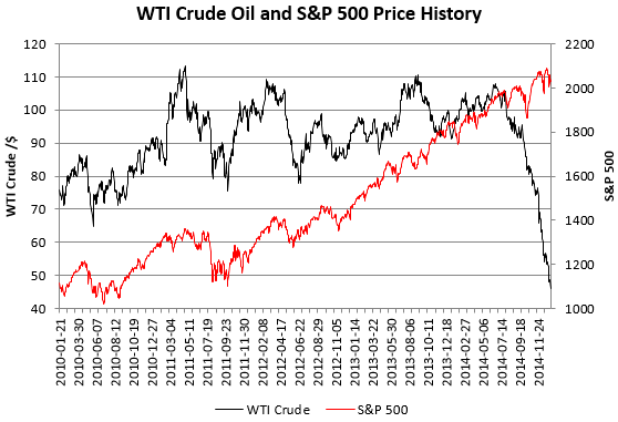
This post will use Apache Spark SQL and DataFrames to query, compare and explore S&P 500, Exxon and Anadarko Petroleum Corporation stock prices for the past 5 years. Stocks and oil prices have a tendency to move together over the past decade as explained in this blog post from Ben Bernanke.

The Spark DataFrames API is designed to make big data processing on tabular data easier. A Spark DataFrame is a distributed collection of data organized into named columns that provides operations to filter, group, or compute aggregates, and can be used with Spark SQL. DataFrames can be constructed from structured data files, existing RDDs, tables in Hive, or external databases. In this post, you’ll learn how to:
- Load data into Spark DataFrames
- Explore data with Spark SQL
This post assumes a basic understanding of Spark concepts. If you have not already read the tutorial on Getting Started with Spark on MapR Sandbox, it would be good to read that first.
Software
This tutorial will run on the MapR Sandbox, which includes Spark
- The examples in this post can be run in the spark-shell, after launching with the spark-shell command.
- You can also run the code as a standalone application as described in the tutorial on Getting Started with Spark on MapR Sandbox.
The Stock Data
We will use stock data from yahoo finance for the following stocks S&P 500 ETF (SPY) , Exxon Mobil Corporation (XOM), and Anadarko Petroleum Corporation (APC) . The following command downloads the stock prices for SPY for the past five years: http://ichart.finance.yahoo.com/table.csv?s=SPY&a=0&b=01&c=2010&d=11&e=31&f=2015&g=d , just change the stock symbol to down load the other 2 files.
The stocks csv files have the following format :
Date,Open,High,Low,Close,Volume,Adj Close
2016-05-18,703.669983,711.599976,700.630005,706.630005,1763400,706.630005
2016-05-17,715.98999,721.52002,704.109985,706.22998,1999500,706.22998
2016-05-16,709.130005,718.47998,705.650024,716.48999,1316200,716.48999
The table below shows the data fields with some sample data:
Using Spark DataFrames we will explore the data with questions like:
- Compute the average closing price per year for SPY, XOM, APC
- Compute the average closing price per month for SPY, XOM, APC
- List the number of times the closing price for SPY went up or down by more than 2 dollars
- Compute the Statistical correllation between XOM and SPY
Loading data into Spark DataFrames
Log into the MapR Sandbox, as explained in Getting Started with Spark on MapR Sandbox, using userid user01, password mapr. Copy the csv data files to your sandbox home directory /user/user01 using scp. Start the spark shell with:
$ spark-shell --master local[*]
First, we will import some packages and instantiate a sqlContext, which is the entry point for working with structured data (rows and columns) in Spark and allows the creation of DataFrame objects.
(In the code boxes, comments are in Green and output is in Blue)
//  SQLContext entry point for working with structured data
val sqlContext = new org.apache.spark.sql.SQLContext(sc)
// Import Spark SQL data types
import sqlContext.implicits._
import sqlContext._
import org.apache.spark.sql.functions._
import org.apache.spark.sql.types._
import org.apache.spark.sql._
import org.apache.spark.mllib.stat.Statistics
Below we use a Scala case class to define the Stock schema corresponding to the csv files for SPY, XOM, and APC. The ParseRDD function applies map() transformations to each line of text in the file to create an RDD of Stock objects.
//define the schema using a case class

case class Stock(dt: String, openprice: Double, highprice: Double, lowprice: Double, closeprice: Double,
  volume: Double, adjcloseprice: Double)

//split a String by comma into an array of Strings, create and return a Stock object from the array
def parseStock(str: String): Stock = {
  val line = str.split(",")
  Stock(line(0), line(1).toDouble, line(2).toDouble, line(3).toDouble, line(4).toDouble, line(5).toDouble,
    line(6).toDouble)
}
//  skip the header, parse each String element in the RDD into a Stock object
def parseRDD(rdd: RDD[String]): RDD[Stock] = {
    val header = rdd.first
    rdd.filter(_(0) != header(0)).map(parseStock).cache()
}
A DataFrame is a distributed collection of data organized into named columns. Spark SQL supports automatically converting an RDD containing case classes to a DataFrame with the method toDF()
// create an RDD of Auction objects
val stocksDF = parseRDD(sc.textFile("spytable.csv")).toDF.cache()
Explore and query the Stock data with Spark DataFrames
DataFrames provide a domain-specific language for structured data manipulation in Scala, Java, and Python; below are some examples with the DataFrames created from the SPY, XOM, and APC stock files. The DataFrame show() action displays the top 20 rows in a tabular form.
// Display the top 20 rows of DataFrame
stocksDF.show()

+----------+----------+----------+----------+----------+----------+-------------+
|        dt| openprice| highprice|  lowprice|closeprice|    volume|adjcloseprice|
+----------+----------+----------+----------+----------+----------+-------------+
|2015-12-31|205.130005|205.889999|203.869995|203.869995|1.148779E8|   201.774586|
|2015-12-30|207.110001|207.210007|205.759995|205.929993| 6.33177E7|    203.81341|
|2015-12-29|206.509995|207.789993|206.470001|207.399994| 9.26407E7|   205.268302|
|2015-12-28|204.860001|205.259995|203.940002|205.210007| 6.58999E7|   203.100824|
|2015-12-24|205.720001|206.330002|205.419998|205.679993| 4.85422E7|    203.56598|
DataFrame printSchema() Prints the schema to the console in a tree format
// Return the schema of this DataFrame
stocksDF.printSchema()
root
 |-- dt: string (nullable = true)
 |-- openprice: double (nullable = false)
 |-- highprice: double (nullable = false)
 |-- lowprice: double (nullable = false)
 |-- closeprice: double (nullable = false)
 |-- volume: double (nullable = false)
 |-- adjcloseprice: double (nullable = false)
Load the data for Exxon and APC:
// Display the top 20 rows of DataFrame
val astocksRDD = parseRDD(sc.textFile("apctable.csv")).cache()
val astocksDF = astocksRDD.toDF().cache
val estocksRDD = parseRDD(sc.textFile("xomtable.csv")).cache()
val estocksDF = estocksRDD.toDF().cache
// Display the top 20 rows of exxon stock
estocksDF.show()

+----------+---------+---------+---------+----------+---------+-------------+
|        dt|openprice|highprice| lowprice|closeprice|   volume|adjcloseprice|
+----------+---------+---------+---------+----------+---------+-------------+
|2015-12-31|77.510002|78.440002|    77.43| 77.949997|1.02855E7|    76.605057|
|2015-12-30|    78.32|78.989998|77.970001| 78.110001|9314600.0|      76.7623|
|2015-12-29|79.989998|80.080002|78.839996| 79.160004|8839000.0|    77.794187|
|2015-12-28|78.120003|78.860001|77.910004| 78.739998|9715800.0|    77.381428|
|2015-12-24|80.269997|80.269997|79.120003| 79.330002|5848300.0|    77.961252|
|2015-12-23|    78.68|80.220001|    78.32| 80.190002|1.51842E7|    78.806414|


// Display the top 20 rows of Anadarko Petroleum stock
astocksDF.show()

+----------+---------+---------+---------+----------+---------+-------------+
|        dt|openprice|highprice| lowprice|closeprice|   volume|adjcloseprice|
+----------+---------+---------+---------+----------+---------+-------------+
|2015-12-31|48.220001|49.049999|47.970001| 48.580002|3672300.0|    48.479166|
|2015-12-30|48.790001|    49.93|48.330002| 48.380001|3534800.0|     48.27958|
|2015-12-29|    50.57|50.880001|49.259998|     49.73|3188000.0|    49.626776|
|2015-12-28|50.220001|    50.57|49.049999| 49.689999|4945200.0|    49.586858|
|2015-12-24|51.400002|51.740002|50.639999| 51.220001|2691600.0|    51.113685|
|2015-12-23|49.549999|51.560001|    48.75|      51.5|8278800.0|    51.393103|
After a dataframe is instantiated, you can query it using SQL queries. Here are some example queries using the Scala DataFrame API:
What was the average closing price per year for S&P?
// Compute the average closing price per year for SPY
stocksDF.select(year($"dt").alias("yr"), $"adjcloseprice").groupBy("yr").avg("adjcloseprice").orderBy(desc("yr")).show

+----+------------------+
|  yr|avg(adjcloseprice)|
+----+------------------+
|2015|201.51264799603175|
|2014|185.20201048809514|
|2013|154.60495069841272|
|2012|127.01593750000006|
|2011|114.27652787698412|
|2010|100.83877198809529|
+----+------------------+
What was the average closing price per year for Exxon?
// Compute the average closing price per year for exxon
estocksDF.select(year($"dt").alias("yr"), $"adjcloseprice").groupBy("yr").avg("adjcloseprice").orderBy(desc("yr")).show

+----+------------------+
|  yr|avg(adjcloseprice)|
+----+------------------+
|2015| 80.01972900000001|
|2014| 91.18927086904760|
|2013| 82.55847863095241|
|2012| 76.89374351599999|
|2011| 69.10707651587303|
|2010| 54.99303160714288|
+----+------------------+
What was the average closing price per month for APC?
// Compute the average closing price per month for apc
astocksDF.select(year($"dt").alias("yr"),month($"dt").alias("mo"), $"adjcloseprice")
  .groupBy("yr","mo").agg(avg("adjcloseprice")).orderBy(desc("yr"),desc("mo")).show

+----+---+------------------+
|  yr| mo|avg(adjcloseprice)|
+----+---+------------------+
|2015| 12| 50.84319331818181|
|2015| 11|       62.84256765|
|2015| 10| 69.07758109090909|
|2015|  9| 65.15292814285712|
|2015|  8| 71.80181557142858|
|2015|  7| 73.94115195454548|
|2015|  6| 81.63433122727272|
|2015|  5|       85.31830925|
You can register a DataFrame as a temporary table using a given name, and then run SQL statements using the sql methods provided by sqlContext. Here are some example queries using sqlContext:
// register the DataFrames as  temp views
stocksDF.registerTempTable("stocks")
estocksDF.registerTempTable("xom")
astocksDF.registerTempTable("apc")


// Calculate and display the average closing price per month for XOM ordered by year,month
// (most recent ones should be displayed first)
sqlContext.sql("SELECT year(xom.dt) as yr, month(xom.dt) as mo,  avg(xom.adjcloseprice)
 as xomavgclose from xom group By year(xom.dt), month(xom.dt) order by year(xom.dt) desc,
 month(xom.dt) desc").show

+----+---+-----------------+
|  yr| mo|      xomavgclose|
+----+---+-----------------+
|2015| 12|76.56664436363636|
|2015| 11|80.34521780000001|
|2015| 10|78.08063068181818|
|2015|  9|71.13764352380952|
|2015|  8|73.75233376190478|
|2015|  7|79.14381290909093|
|2015|  6|81.60600477272729|
. . .
When did the closing price for SPY go up or down by more than 2 dollars?
// List when the closing price for SPY went up or down by more than 2 dollars
var res = sqlContext.sql("SELECT spy.dt, spy.openprice, spy.closeprice, abs(spy.closeprice - spy.openprice)
   as spydif FROM spy WHERE abs(spy.closeprice - spy.openprice) > 4 ")
res.show

+----------+----------+----------+-----------------+
|        dt| openprice|closeprice|           spydif|
+----------+----------+----------+-----------------+
|2015-12-04|205.610001|209.619995|4.009993999999978|
|2015-10-02|189.770004|     195.0|         5.229996|
|2015-09-09|199.320007|194.789993|4.530013999999994|
|2015-08-25|195.429993|187.270004|8.159988999999996|
|2015-01-28|204.169998|200.139999|4.029999000000004|
|2011-08-11|113.260002|117.330002|4.069999999999993|
|2011-08-08|116.910004|112.260002|4.650002000000001|
When did the closing price for SPY AND XOM go up or down by more than 2 dollars?
// List  when  the closing price for SPY AND XOM went up or down by more than 2 dollars
sqlContext.sql("SELECT spy.dt, abs(spy.closeprice - spy.openprice) as spydif, xom.dt,
 abs(xom.closeprice - xom.openprice) as xomdif FROM spy join xom on spy.dt = xom.dt
 WHERE (abs(spy.closeprice - spy.openprice) > 2 and abs(xom.closeprice - xom.openprice) > 2)").show

+----------+------------------+----------+------------------+
|        dt|            spydif|        dt|            xomdif|
+----------+------------------+----------+------------------+
|2011-08-08| 4.650002000000001|2011-08-08| 2.549995999999993|
|2015-08-25| 8.159988999999996|2015-08-25| 2.599998999999997|
|2014-07-31|2.5200049999999976|2014-07-31|3.0400009999999895|
|2014-10-16| 3.210005999999993|2014-10-16| 2.019996000000006|
|2015-10-02|          5.229996|2015-10-02|          2.489998|
|2015-10-22|2.2799990000000037|2015-10-22|2.2099989999999963|
|2015-11-16| 3.299987999999985|2015-11-16|2.9599999999999937|
|2015-01-16| 2.860001000000011|2015-01-16|2.1400000000000006|
|2013-02-25|3.6300050000000113|2013-02-25| 2.180000000000007|
+----------+------------------+----------+------------------+
What was the max, min closing price for SPY and XOM by Year?
// What was the max, min closing price for SPY and XOM by Year?
sqlContext.sql("SELECT year(spy.dt) as yr, max(spy.adjcloseprice), min(spy.adjcloseprice),
  max(xom.adjcloseprice), min(xom.adjcloseprice) FROM spy join xom on spy.dt = xom.dt
  group By year(spy.dt)").show

+----+------------------+------------------+------------------+------------------+
|  yr|max(adjcloseprice)|min(adjcloseprice)|max(adjcloseprice)|min(adjcloseprice)|
+----+------------------+------------------+------------------+------------------+
|2015|        208.078387|        183.295739|         89.383483|         66.940931|
|2013|        175.663503|        135.696272|         93.790574|         77.915206|
|2014|        202.398157|        165.657652|         97.784793|         82.102662|
|2012|        135.581384|        116.289598|         83.553047|         68.911556|
|2010|        112.488545|         90.337415|         62.909315|         47.826016|
|2011|        122.406931|         99.632548|         75.782221|         59.319652|
+----+------------------+------------------+------------------+------------------+
The physical plan for DataFrames
Unlike the basic Spark RDD API, the interfaces provided by Spark SQL provide Spark with more information about the structure of both the data and the computation being performed. Internally, Spark SQL uses this extra information to perform optimizations in the execution plan.
The Catalyst query optimizer creates the physical Execution Plan for DataFrames as shown in the diagram below:
Print the Physical Plan to the Console
DataFrames are designed to take the SQL queries constructed against them and optimize the execution as sequences of Spark Jobs as required. You can print the physical plan for a DataFrame using the explain operation as shown below:
//  Prints the physical plan to the console for debugging purpose
sqlContext.sql("SELECT spy.dt, spy.openprice, spy.closeprice, abs(spy.closeprice - spy.openprice) as spydif FROM spy WHERE abs(spy.closeprice - spy.openprice) > 4 ").explain

== Physical Plan ==
*Project [dt#84, openprice#85, closeprice#88, abs((closeprice#88 - openprice#85)) AS spydif#908]
+- *Filter (abs((closeprice#88 - openprice#85)) > 4.0)
   +- InMemoryTableScan [dt#84, openprice#85, closeprice#88], [(abs((closeprice#88 - openprice#85)) > 4.0)]
      :  +- InMemoryRelation [dt#84, openprice#85, highprice#86, lowprice#87, closeprice#88, volume#89, adjcloseprice#90], true, 10000, StorageLevel(disk, memory, deserialized, 1 replicas)
      :     :  +- Scan ExistingRDD[dt#84,openprice#85,highprice#86,lowprice#87,closeprice#88,volume#89,adjcloseprice#90]
Join Spy , XOM, APC in order to compare closing prices
// Join all stock closing prices in order to  compare
val joinclose=sqlContext.sql("SELECT apc.dt, apc.adjcloseprice as apcclose, spy.adjcloseprice as spyclose, xom.adjcloseprice as xomclose from apc join spy on apc.dt = spy.dt join xom on spy.dt = xom.dt").cache
joinclose.show
joinclose.registerTempTable("joinclose")

+----------+---------+----------+---------+
|        dt| apcclose|  spyclose| xomclose|
+----------+---------+----------+---------+
|2015-12-31|48.479166|201.774586|76.605057|
|2015-12-30| 48.27958| 203.81341|  76.7623|
|2015-12-29|49.626776|205.268302|77.794187|
|2015-12-28|49.586858|203.100824|77.381428|
|2015-12-24|51.113685| 203.56598|77.961252|
|2015-12-23|51.393103|203.902497|78.806414|
|2015-12-22|48.449225|201.408393|76.310238|
|2015-12-21|46.453377|199.597201|75.926968|
|2015-12-18|45.575202|197.964166|75.946619|
Get year average closing prices for XOM, SPY, APC
// get year average closing prices
sqlContext.sql("SELECT year(joinclose.dt) as yr, avg(joinclose.apcclose) as avgapcclose,
   avg(joinclose.spyclose) as avgspyclose, avg(joinclose.xomclose) as avgxomclose from joinclose
   group By year(joinclose.dt) order by year(joinclose.dt)").show

+----+------------------+------------------+-----------------+
|  yr|       avgapcclose|       avgspyclose|      avgxomclose|
+----+------------------+------------------+-----------------+
|2010|56.993713151840936|100.83877197144524|54.99303162287152|
|2011|  73.1128199895223|114.27652791946653|69.10707661462209|
|2012| 70.31488655090332|127.01593780517578|76.89374353027344|
|2013| 84.43673639448862|154.60495104108537|82.55847873384991|
|2014| 92.59866605486188|185.20201020013718|91.18927077641563|
|2015| 74.17173276628766|201.51264778016105|80.01972888764881|
+----+------------------+------------------+-----------------+
Save the joined view to a parquet table for later use. Saving tables in parquet format is a good choice, because it is a compressed format and querying parquet files is faster than txt files because it is a columnar storage format.
// save joined view in a parquet table
joinclose.write.format("parquet").save("joinstock.parquet")
Read the parquet table into a dataframe.
// read  parquet table into a dataframe
val df = sqlContext.read.parquet("joinstock.parquet")
df.show

+----------+----------+----------+---------+
|        dt|  apcclose|  spyclose| xomclose|
+----------+----------+----------+---------+
|2010-12-28| 66.210166|112.408148|62.909315|
|2011-02-18| 77.506863|120.180146|72.784694|
|2011-11-18| 73.691167|110.553793| 68.33066|
|2012-04-11| 71.608401|125.501915|72.938063|

df.printSchema

root
 |-- dt: string (nullable = true)
 |-- apcclose: double (nullable = true)
 |-- spyclose: double (nullable = true)
 |-- xomclose: double (nullable = true)
What is the average closing for all 3 by month ?
// What is the average closing for all 3 by month ?
df.select(year($"dt").alias("yr"),month($"dt").alias("mo"), $"apcclose", $"xomclose",$"spyclose").groupBy("yr","mo").agg(avg("apcclose"),avg("xomclose"),avg("spyclose")).orderBy(desc("yr"),desc("mo")).show

+----+---+------------------+-----------------+------------------+
|  yr| mo|     avg(apcclose)|    avg(xomclose)|     avg(spyclose)|
+----+---+------------------+-----------------+------------------+
|2015| 12| 50.84319331818181|76.56664436363636|202.76129027272725|
|2015| 11|       62.84256765|       80.3452178|      205.00676435|
|2015| 10| 69.07758109090909|78.08063068181818|199.11801163636366|
|2015|  9| 65.15292814285715|71.13764352380952|190.92923485714286|
|2015|  8| 71.80181557142856|73.75233376190477|199.94614619047618|
|2015|  7| 73.94115195454546|79.14381290909091| 204.8488672272727|
|2015|  6| 81.63433122727272|81.60600477272727|205.05149654545457|
|2015|  5|       85.31830925|83.83634099999999|      205.87453735|
|2015|  4| 89.53835657142857|82.72748161904762|203.88186028571428|
|2015|  3| 80.24251268181818|81.54228986363636|202.16996027272728|
|2015|  2| 83.92761210526317|86.76038289473684|201.99138773684209|
|2015|  1|        77.5413219|86.01301014999999|196.44655274999997|
|2014| 12| 78.14734299999999|87.14667045454546|198.69392127272724|
|2014| 11| 88.66765210526316|90.34088715789476|197.38651600000003|
|2014| 10| 89.61032617391305|87.81811986956522|186.71991460869566|
|2014|  9|103.89716504761905|91.23819252380953| 191.8662882857143|
|2014|  8| 106.5734889047619| 93.3404890952381| 188.4780800952381|
|2014|  7|105.87142745454547| 96.2867429090909| 189.2690632727273|


// Print the physical plan to the console with Explain
df.select(year($"dt").alias("yr"),month($"dt").alias("mo"), $"apcclose", $"xomclose",$"spyclose").groupBy("yr","mo").agg(avg("apcclose"),avg("xomclose"),avg("spyclose")).orderBy(desc("yr"),desc("mo")).explain

== Physical Plan ==
*Sort [yr#6902 DESC, mo#6903 DESC], true, 0
+- Exchange rangepartitioning(yr#6902 DESC, mo#6903 DESC, 200)
   +- *HashAggregate(keys=[yr#6902, mo#6903], functions=[avg(apcclose#6444), avg(xomclose#6446), avg(spyclose#6445)])
      +- Exchange hashpartitioning(yr#6902, mo#6903, 200)
         +- *HashAggregate(keys=[yr#6902, mo#6903], functions=[partial_avg(apcclose#6444), partial_avg(xomclose#6446), partial_avg(spyclose#6445)])
            +- *Project [year(cast(dt#6443 as date)) AS yr#6902, month(cast(dt#6443 as date)) AS mo#6903, apcclose#6444, xomclose#6446, spyclose#6445]
               +- *BatchedScan parquet [dt#6443,apcclose#6444,spyclose#6445,xomclose#6446] Format: ParquetFormat, InputPaths: dbfs:/joinstock.parquet, PushedFilters: [], ReadSchema: struct
Is there a Statistical correllation between Exxon Stock Prices and the S&P ?
// Calculate the correlation between the  two series of data
val seriesX = df.select( $"xomclose").map{row:Row => row.getAs[Double]("xomclose") }.rdd
val seriesY = df.select( $"spyclose").map{row:Row => row.getAs[Double]("spyclose")}.rdd
val correlation = Statistics.corr(seriesX, seriesY, "pearson")

correlation: Double = 0.7867605093839455
Is there a Statistical correllation between Exxon Stock Prices and APC ?
// Calculate the correlation between the  two series of data
val seriesX = df.select( $"xomclose").map{row:Row => row.getAs[Double]("xomclose") }.rdd
val seriesY = df.select( $"apcclose").map{row:Row => row.getAs[Double]("apcclose") }.rdd
val correlation = Statistics.corr(seriesX, seriesY, "pearson")

correlation: Double = 0.8140740223956957
Summary
In this blog post, you’ve learned how to load data into Spark DataFrames, and explore data with Spark SQL. If you have any further questions, or want to share how you are using Spark DataFrames, please add your comments in the section below.
Want to learn more?
- Spark SQL and DataFrame Guide
- Free On Demand Spark Training
- Apache Spark
- Apache Spark Resources in Converge Community
| Reference: | Using Apache Spark SQL to Explore S&P 500, and Oil Stock Prices from our JCG partner Carol McDonald at the Mapr blog. |


