Push your configuration to the limit – spice it up with statistics

Gal LevinskyMarch 10th, 2016Last Updated: March 10th, 2016

0 40 6 minutes read

So – you built a service with an advanced algorithm that uses some kind of classification in order to detect certain events – How would you know your configuration data is optimal? How would you measure the impact on accuracy each time the algorithm is changed?

The following post will show you how to use a mixture of concepts from Machine Learning, Statistics & Operations Research in order to maximize configuration set of an algorithm.

This method is highly efficient in a client-side classification mechanism that requires accuracy but lacking learning time or processing power to do it.

The suggested method is divided into 4 phases:

Test data preparation
Running the test
Result measurement
Analysis
Determine the winner

Test data preparation

Prepare a CSV file with data that have an indication of its correctness. e.g. if the algorithm should detect cars, we would have a data such as:

Toyota,1
mouse,0
Nissan,1
keyboard,0
Ford,1
button,0

Where 0 is an indication that the data is not a car and 1 is an indication that the data is a car.

The amount of data set will be discussed later on and might deserve a separate post, however, for simplification, assume we have 10 tests with 5 correct data and 5 incorrect data.

Running the test

Building a test to send data to your algorithm

The overall concept is clear:

Read the test data
Send it to your algorithm
Record the result (i.e. whether the algorithm identified the data correctly)

However, since we want to find out the optimal configuration we shall add additional step, before sending the data to the algorithm:

Set the algorithm with a certain configuration, meaning that the parameters your algorithm use would be able to be configured, for each run.

So the high level run steps should be:

Read the test data
Prepare algorithm configuration permutations
Send the data to your algorithm for each configuration permutation
Record the result for each run

Few things to note:

Your algorithm should always return a result whether it identified the data or not, so you could record true negative and false negative.
Externalize your configuration, enable to set it from outer class, as it required to do with each configuration set.
Shuffle the test data between each run & execute multiple runs per specific configuration set. Shuffling the data will enable to reduce correlation to the data order, executing multiple runs with the same configuration will help reduce any random standard deviation.

Result measurement

When your test gets the data back from the algorithm compare the algorithm predicted condition (positive/negative) versus the true condition, based on the indication in the test data.

Make sure to count the following:

TruePositive (TP) = correctly identified, a hit!
Classified correctly as positive
True negative (TN) = correctly rejected, equivalent to correct rejection
Classified correctly as negative
False positive (FP) = incorrectly identified, equivalent to false alarm (type I error)
Classified wrongly as positive
False negative (FN) = incorrectly rejected, a miss (type II error)
Classified wrongly as negative

The algorithm accuracy would be measured as follow:

Accuracy (ACC) = (TP + TN)/(TP + FP + FN + TN)

I like also to measure the following:

True Positive Rate (TPR), also known as sensitivity: TPR = TP/(TP + FP), If all your positive data were identified correctly, the value would be 1, so as closer the result is to 1 – the better.
True Negative Rate, also known as specificity: NPV = TN/(TN+FN), If all the negative data were identified correctly, the value would be 1, so as closer the result is to 1 – the better.
False Positive Rate (FPR), also known as fall-outs: FPR = FP/(FP + TN), The closer the value is to 0, means fewer false alarm.
False Negative Rate (FNR): FNR = FN/(TP+FN), The closer the value is to 0, means fewer missed out.

Cost function

Highly important.

This is where you quantify the statistical analysis and the results into a single score that will help to determine how good the overall run/configuration is and will also make it simpler to compare between runs.

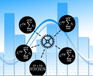
The cost function formula would look as follows:

Where CTP Is the cost of True Positive results, CTN is the cost of True Negative results and so on.

In a simplified manner, you need to sum each occurrence based on a certain weight.

You need to decide how much weight to give each data result, i.e. the value of TP, TN, FP & FN.

This may vary for each customer need, for example, some customers would like your algorithm to provide more results at the expense of quality, so you would give less penalty/weight on FP / FN result. Others would be very sensitive to faulty results, so your cost function would give higher value/weight to FP.

Note: I would recommend setting the cost value of TP and TN as such that if all the results are correct the expected sum value would be round number. For example, if we have 10 tests, 5 positive and 5 negatives, we would give each TP & TN the cost value of 10, so the overall score of a fully successful run would be 100.

Save in a file the configuration permutation and its score.

Analysis

Put all the run result in excel.

It is very easy to find the maximum cost function score and its configuration set, however, to find the most robust configuration, find the configuration value which had the best average across other permutations. To do this create a pivot table where all the configuration values are in the “Rows” section and the drag the cost function score field into the “Sum Value” section. Duplicate the score field in the “Sum Value” section and set one as an average function and the other as Max function.

Since all the configuration set is in the Rows section in the pivot table, it is possible to aggregate it so only the first value is shown.

The final step is to write the best value per average score. Sometimes the a certain configuration value best average score would match the best maximum score, however, sometimes it won’t.

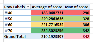
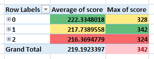
In the below images you can see a demonstration of a certain configuration value and its average and maximum score. You could see that not always there is a correlation between average and maximum score.

In the below image a certain algorithm configuration has values 40,50,60 & 70.

The value 70 appears in the configuration permutation of the maximum score and also has the best average. Having the best average means that setting the value 70 would give the best average score for any other configuration permutations. It implies about the robustness of this configuration.

In the below image we choose another algorithm configuration parameter with the values of 0,1 & 2.

We did it by dragging the relevant configuration parameter field in the pivot table “Rows” section to the first position.

You can see that the best average cost function score is for value 0 and the best maximum cost function score is for the value 1.

Determine the winner with a final contest

At the end of the analysis phase, you would have a configuration set that provides the maximum score and a configuration set that provide the best average score.

This phase will try to minimize any implication the algorithm might have due to the test data, i.e. we want to rule out the possibility the algorithm is biased to a certain test data.

Create a test data with the following:

80% positive tests
70% positive tests
30% positive tests
20% positive tests

Execute each test data on each of the maximum and average configuration set.

The winner would be based on your customer need and the given result. If there isn’t much variation between the runs score, it means that your algorithm is robust and you can choose the one that gave you maximum score, however, if there is big variation, it means that your algorithm is data dependent and it up to your customer needs whether to choose the best average or the best maximum.

An extra bonus getting using this method:

Test how your algorithm utilized resources over time (Memory leaks, CPU utilization, disk space,..)
Enable to accurately measure changes in the algorithm over time, across versions.

Any feedback is highly welcome.